Example 4: Site Response Analysis with Deconvolution Using TransferFunction Tool
Overview
This example demonstrates the deconvolution capability of the TransferFunction class in Femora. Building upon Example 2’s multi-layered soil profile, this example shows how to:
Start with a recorded surface motion (Ricker wavelet)
Use the
TransferFunctiontool to deconvolve and compute the corresponding bedrock motionApply the computed bedrock motion as input to a numerical site response analysis
Verify that the numerical model reproduces the original surface motion
This workflow is particularly valuable for creating Domain Reduction Method (DRM) datasets and validating site response models against recorded surface motions.
Schematic representation of the deconvolution workflow: from surface motion to bedrock motion and back to surface
Model Description
Soil Profile:
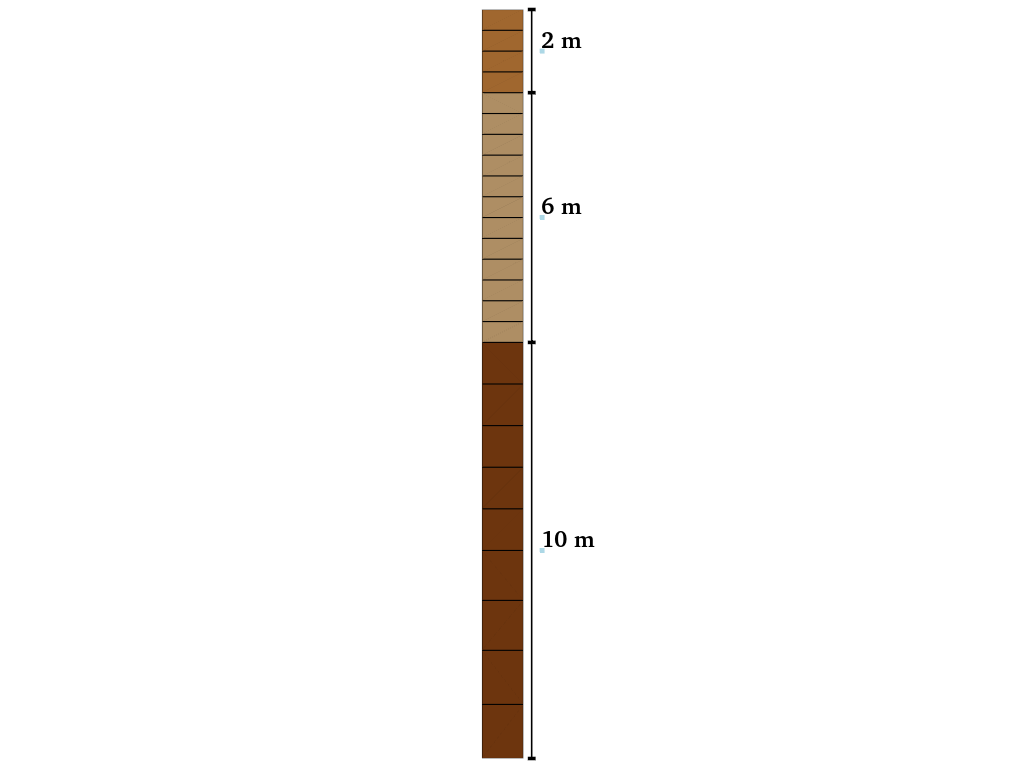
This example uses the same three-layer soil profile as Example 2:
Layer 1 (Bottom): 10m thick - Stiff material (Vs = 262.5 m/s)
Layer 2 (Middle): 6m thick - Medium stiffness material (Vs = 196.3 m/s)
Layer 3 (Top): 2m thick - Soft material (Vs = 144.3 m/s)
All material properties, including Rayleigh damping parameters, are identical to Example 2.
Input Motion:
Unlike previous examples that used frequency sweep inputs, this example uses a Ricker wavelet recorded at the surface. The Ricker wavelet provides a realistic broadband signal that is commonly used in seismic analysis.
Deconvolution Process
The key innovation in this example is the use of Femora’s TransferFunction class to perform deconvolution. The process is implemented in the deconvolve.py script:
Loading Surface Motion
First, we load the recorded surface motion using the TimeHistory class:
from femora.tools.transferFunction import TransferFunction, TimeHistory

# Load the surface motion (Ricker wavelet)
record = TimeHistory.load(acc_file="ricker_surface.acc",
                          time_file="ricker_surface.time",
                          unit_in_g=True,
                          gravity=9.81)
Defining Soil Profile
The soil profile is defined with the same properties as Example 2:
soil = [
    {"h": 2,  "vs": 144.2535646321813, "rho": 19.8*1000/9.81, "damping": 0.03,
     "damping_type":"rayleigh", "f1": 2.76, "f2": 13.84},
    {"h": 6,  "vs": 196.2675276462639, "rho": 19.1*1000/9.81, "damping": 0.03,
     "damping_type":"rayleigh", "f1": 2.76, "f2": 13.84},
    {"h": 10, "vs": 262.5199305117452, "rho": 19.9*1000/9.81, "damping": 0.03,
     "damping_type":"rayleigh", "f1": 2.76, "f2": 13.84},
]
rock = {"vs": 8000, "rho": 2000.0, "damping": 0.00}
Performing Deconvolution
The deconvolution is performed using the _deconvolve method of the TransferFunction class:
# Create transfer function instance
tf = TransferFunction(soil, rock, f_max=50.0)

# Deconvolve to get bedrock motion
bedrock = tf._deconvolve(time_history=record)

# Save the computed bedrock motion
np.savetxt("ricker_base.acc", bedrock.acceleration, fmt='%.6f')
np.savetxt("ricker_base.time", bedrock.time, fmt='%.6f')

# Generate comparison plots
fig = tf.plot_deconvolved_motion(time_history=record)
The _deconvolve method works by:
Converting the surface time history to frequency domain
Applying the inverse of the transfer function to remove site amplification effects
Converting back to time domain to obtain the bedrock motion
Numerical Verification
The computed bedrock motion is then used as input to the same numerical model as Example 2. The numerical model applies uniform excitation at the base of the soil column using the deconvolved bedrock motion.
Model Setup:
The numerical model setup is identical to Example 2, with the key difference being the input motion source. Instead of using a frequency sweep, the model uses the computed bedrock acceleration as the base excitation.
Expected Results:
If the deconvolution and numerical modeling are accurate, the surface motion computed by the numerical model should closely match the original recorded surface motion that was used for deconvolution.
Results and Analysis
Transfer Function Comparison
The transfer function comparison demonstrates the accuracy of the deconvolution process:
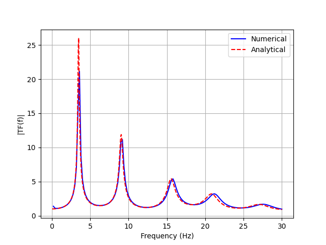
Comparison of analytical transfer function with numerical results from the deconvolved motion
Time History Comparison
The most important validation is the comparison between time histories:
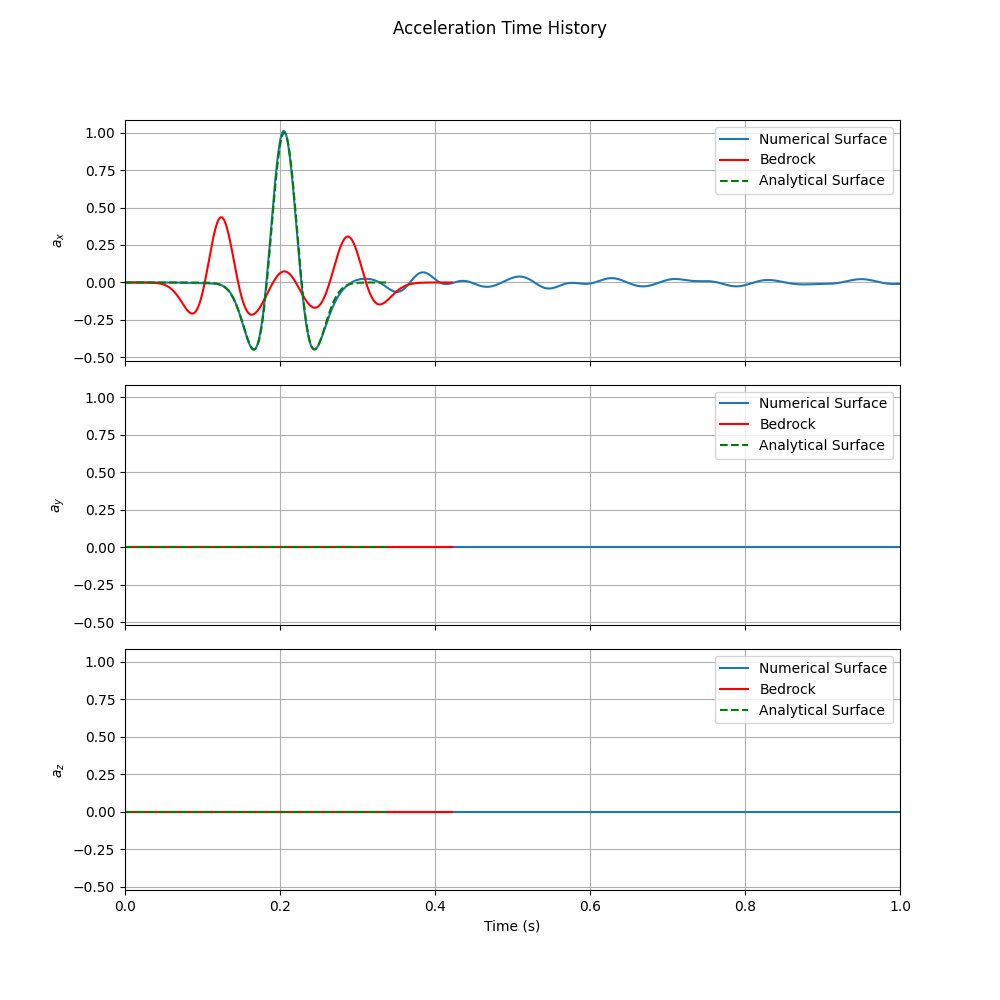
Comparison of time histories: original surface motion (used for deconvolution), computed bedrock motion, and numerical surface response
This figure shows three key time histories:
Numerical Surface Response (blue): The surface motion computed by applying the bedrock motion to the numerical model
Computed Bedrock Motion (red): The result of deconvolving the surface motion
Original Surface Motion (green): The Ricker wavelet recorded at the surface
The excellent agreement between the original surface motion and the numerical surface response validates both the deconvolution process and the numerical model accuracy.
Simulation Visualization
This animation demonstrates the wave propagation from bedrock to surface using the deconvolved input motion, showing how the original surface motion is reproduced through the soil layers.
Applications and Benefits
Model Validation:
The deconvolution process provides a powerful tool for validating site response models. By comparing the forward-modeled surface response with the original recorded motion, you can assess the accuracy of your soil profile characterization and modeling assumptions.
Practical Workflow:
Obtain recorded surface motions from seismic stations
Characterize the local soil profile (layering, properties)
Use deconvolution to compute equivalent bedrock motion
Apply bedrock motion to detailed numerical models
Validate results against recorded surface motion
Conclusion
This example demonstrates:
The practical application of the
TransferFunctionclass for deconvolutionHow to create realistic bedrock motions from surface recordings
The validation of numerical models through time history comparison
A complete workflow for site-specific seismic analysis
The deconvolution capability in Femora provides a bridge between recorded seismic data and numerical modeling, enabling more realistic and validated site response analyses.
Code Access
The full source code for this example is available in the Femora repository:
Example directory:
examples/SiteResponse/Example4/Deconvolution script:
examples/SiteResponse/Example4/deconvolve.pyNumerical model script:
examples/SiteResponse/Example4/femoramodel.pyPost-processing script:
examples/SiteResponse/Example4/plot.py
The deconvolution script is the key component of this example:
import os
import femora as fm
os.chdir(os.path.dirname(__file__))


# create one damping for all the meshParts
uniformDamp = fm.damping.frequencyRayleigh(f1 = 2.76, f2 = 13.84, dampingFactor=0.03)
region = fm.region.elementRegion(damping=uniformDamp)

# defining the mesh parts
Xmin = 0.0 ;Xmax = 1.0
Ymin = 0.0 ;Ymax = 1.0
Zmin = -18.;Zmax = 0.0
dx   = 1.0; dy   = 1.0
Nx = int((Xmax - Xmin)/dx)
Ny = int((Ymax - Ymin)/dy)


layers_properties = [
    {"user_name": "Dense Ottawa1",  "G": 145.0e6, "gamma": 19.9,  "nu": 0.3, "thickness": 2.6, "dz": 1.3},
    {"user_name": "Dense Ottawa2",  "G": 145.0e6, "gamma": 19.9,  "nu": 0.3, "thickness": 2.4, "dz": 1.2},
    {"user_name": "Dense Ottawa3",  "G": 145.0e6, "gamma": 19.9,  "nu": 0.3, "thickness": 5.0, "dz": 1.0},
    {"user_name": "Loose Ottawa",   "G": 75.0e6,  "gamma": 19.1,  "nu": 0.3, "thickness": 6.0, "dz": 0.5},
    {"user_name": "Dense Montrey",  "G": 42.0e6,  "gamma": 19.8,  "nu": 0.3, "thickness": 2.0, "dz": 0.5}
]


for layer in layers_properties:
    name = layer["user_name"]
    nu   = layer["nu"]
    rho  = layer["gamma"] * 1000 / 9.81        # Density in kg/m^3
    Vs   = (layer["G"] / rho) ** 0.5           # Shear wave velocity in m/s
    E    = 2 * layer["G"] * (1 + layer["nu"])  # Young's modulus in Pa
    E    = E / 1000.                           # Convert to kPa
    rho  = rho / 1000.                         # Convert to kg/m^3

    print(f"Layer: {name}, Vs: {Vs}")


    # Define the material
    fm.material.create_material(material_category="nDMaterial", material_type="ElasticIsotropic", user_name=name, E=E, nu=nu, rho=rho)

    # Define the element
    ele = fm.element.create_element(element_type="stdBrick", ndof=3, material=name, b1=0.0, b2=0.0, b3=0)

    fm.meshPart.create_mesh_part(category="Volume mesh", mesh_part_type="Uniform Rectangular Grid",
                                 user_name=name, element=ele, region=region,
                                **{
                                    'X Min': Xmin, 'X Max': Xmax,
                                    'Y Min': Ymin, 'Y Max': Ymax,
                                    'Z Min': Zmin, 'Z Max': Zmin + layer["thickness"],
                                    'Nx Cells': Nx, 'Ny Cells': Ny, 'Nz Cells': int(layer["thickness"] / layer["dz"])
                                })
    Zmin += layer["thickness"]


# #  Create assembly Sections
fm.assembler.create_section(meshparts=[layer["user_name"] for layer in layers_properties], num_partitions=0)


# Assemble the mesh parts
fm.assembler.Assemble()

# Create a TimeSeries for the uniform excitation
timeseries = fm.timeSeries.create_time_series(series_type="path",
                                              filePath="ricker_base.acc",
                                              fileTime="ricker_base.time",
                                              factor= 9.81)

# Create a pattern for the uniform excitation
kobe = fm.pattern.create_pattern(pattern_type="uniformexcitation",dof=1, time_series=timeseries)


# boundary conditions
fm.constraint.mp.create_laminar_boundary(bounds=(-17.9,0),dofs=[1,2,3], direction=3)
fm.constraint.sp.fixMacroZmin(dofs=[1,1,1],tol=1e-3)


# Create a recorder for the whole model
mkdir = fm.actions.tcl("file mkdir Results")
recorder = fm.recorder.create_recorder("vtkhdf", file_base_name="Results/result.vtkhdf",resp_types=["accel", "disp", "vel"], delta_t=0.001)

# gravity analysis
newmark_gamma = 0.6
newnark_beta = (newmark_gamma + 0.5)**2 / 4
system = fm.analysis.system.bandGeneral()
numberer = fm.analysis.numberer.rcm()
dampNewmark = fm.analysis.integrator.newmark(gamma=newmark_gamma, beta=newnark_beta)
gravity = fm.analysis.create_default_transient_analysis(username="gravity",
                                                        dt=1.0, num_steps=30,
                                                        options={"system": system,
                                                                 "numberer": numberer,
                                                                 "integrator": dampNewmark})

# dynamic analysis
dynamic = fm.analysis.create_default_transient_analysis(username="dynamic",
                                                        final_time=5.0, dt=0.001,
                                                        options={"system": system,
                                                                 "numberer": numberer})


reset = fm.actions.seTime(pseudo_time=0.0)

# Add the recorder and gravity analysis step to the process
fm.process.add_step(gravity,  description="Gravity Analysis Step")
fm.process.add_step(kobe,     description="Uniform Excitation (Kobe record)")
fm.process.add_step(mkdir,    description="Create Results Directory")
fm.process.add_step(recorder, description="Recorder of the whole model")
fm.process.add_step(reset,    description="Reset pseudo time")
fm.process.add_step(dynamic,  description="Dynamic Analysis Step")
fm.export_to_tcl("mesh.tcl")


# fm.gui()