Example 3: 3D Multi-Processor Site Response Analysis
Overview
This example extends Example 2 by transforming the single-column model into a full 3D domain that can be distributed across multiple processors. While site response is inherently a 1D problem, this example demonstrates:
How to create wider 3D models with multiple elements in the horizontal plane
How to configure parallel processing for larger models
That the 1D response remains consistent even with 3D domain modeling
How to process and visualize the results of multi-processor simulations
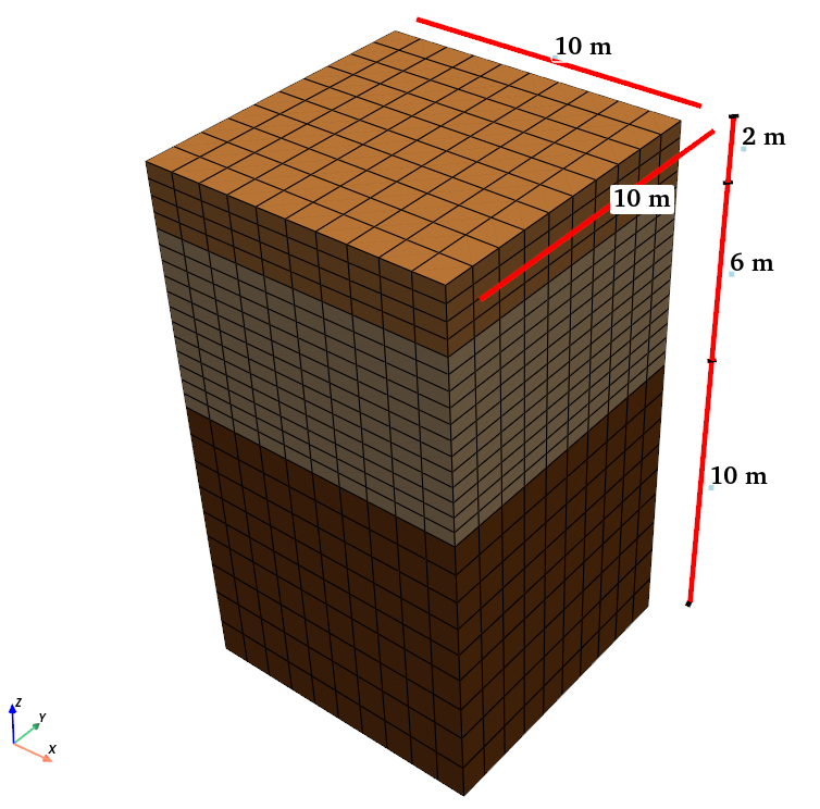
3D multi-processor site response model with 10×10m horizontal dimensions
Model Description
Soil Domain:
10m × 10m soil domain in horizontal dimensions (compared to 1×1m in Examples 1-2)
Total depth of 18m (identical to previous examples)
Three distinct soil layers with the same material properties as Example 2
Parallel Configuration:
Domain partitioned across 8 processors
Automatic domain decomposition for load balancing
Synchronized at layer interfaces for wave propagation continuity
Analysis Setup:
The frequency sweep input, boundary conditions, material properties, and damping setup remain identical to Example 2, ensuring comparable results with the previous examples.
Implementation Details
Let’s focus on the key differences in implementation from the previous examples:
3D Domain Configuration
The most significant difference is the expanded horizontal dimensions, creating a true 3D domain:
# Expanded horizontal dimensions
Xmin = -5.0 ;Xmax = 5.0
Ymin = -5.0 ;Ymax = 5.0
Zmin = -18.;Zmax = 0.0
dx   = 1.0; dy   = 1.0
Nx = int((Xmax - Xmin)/dx)
Ny = int((Ymax - Ymin)/dy)
This creates a 10×10m horizontal domain (with 10 elements in each direction) instead of the 1×1m domain used in previous examples.
Layer and Material Definition
The layer definitions remain similar to Example 2, but we use a more concise approach to define and create all layers in a single loop:
layers_properties = [
    {"user_name": "Dense Ottawa1",  "G": 145.0e6, "gamma": 19.9,  "nu": 0.3, "thickness": 2.6, "dz": 1.3},
    {"user_name": "Dense Ottawa2",  "G": 145.0e6, "gamma": 19.9,  "nu": 0.3, "thickness": 2.4, "dz": 1.2},
    {"user_name": "Dense Ottawa3",  "G": 145.0e6, "gamma": 19.9,  "nu": 0.3, "thickness": 5.0, "dz": 1.0},
    {"user_name": "Loose Ottawa",   "G": 75.0e6,  "gamma": 19.1,  "nu": 0.3, "thickness": 6.0, "dz": 0.5},
    {"user_name": "Dense Montrey",  "G": 42.0e6,  "gamma": 19.8,  "nu": 0.3, "thickness": 2.0, "dz": 0.5}
]

for layer in layers_properties:
    name = layer["user_name"]
    nu   = layer["nu"]
    rho  = layer["gamma"] * 1000 / 9.81        # Density in kg/m^3
    Vs   = (layer["G"] / rho) ** 0.5           # Shear wave velocity in m/s
    E    = 2 * layer["G"] * (1 + layer["nu"])  # Young's modulus in Pa
    E    = E / 1000.                           # Convert to kPa
    rho  = rho / 1000.                         # Convert to kg/m^3

    # Define material and element for each layer
    fm.material.create_material(material_category="nDMaterial",
                              material_type="ElasticIsotropic",
                              user_name=name, E=E, nu=nu, rho=rho)

    ele = fm.element.create_element(element_type="stdBrick", ndof=3,
                                  material=name, b1=0.0, b2=0.0, b3=-9.81 * rho)

    # Create mesh part for the layer
    fm.meshPart.create_mesh_part(category="Volume mesh",
                               mesh_part_type="Uniform Rectangular Grid",
                               user_name=name, element=ele, region=region,
                               **{
                                  'X Min': Xmin, 'X Max': Xmax,
                                  'Y Min': Ymin, 'Y Max': Ymax,
                                  'Z Min': Zmin, 'Z Max': Zmin + layer["thickness"],
                                  'Nx Cells': Nx, 'Ny Cells': Ny,
                                  'Nz Cells': int(layer["thickness"] / layer["dz"])
                               })
    Zmin += layer["thickness"]
Parallel Processing Configuration
The key difference in this example is the parallel processing setup. Instead of specifying num_partitions=0 as in Example 1, we use num_partitions=8 to distribute the model across 8 processors:
# Configure for parallel processing with 8 partitions
fm.assembler.create_section(meshparts=[layer["user_name"] for layer in layers_properties],
                         num_partitions=8)

# Assemble the mesh parts
fm.assembler.Assemble()
This setup automatically partitions the domain for parallel execution. For larger models, this significantly reduces computation time.
Analysis System and Equations
Unlike Example 1 which specified serial solvers, Example 3 uses the default parallel solvers in Femora:
# Dynamic analysis with default parallel solvers
dynamic = fm.analysis.create_default_transient_analysis(username="dynamic",
                                                    final_time=40.0, dt=0.001)
The parallel configuration automatically selects appropriate solvers and equation numbering schemes for distributed computation.
Results and Analysis
Despite the significantly larger domain and parallel execution, the results remain essentially identical to Example 2. This demonstrates that:
The site response problem remains one-dimensional in nature
The parallel implementation correctly maintains wave propagation physics
The transfer function approach is valid regardless of horizontal domain size
Transfer Function Comparison
The transfer function calculated from the 3D model’s surface response shows excellent agreement with both the analytical solution and the single-column model from Example 2:
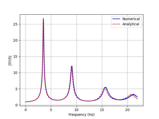
Comparison of numerical (from 3D model) and analytical transfer functions
The only noticeable differences are minor numerical artifacts due to the domain decomposition and parallel execution, but these differences are negligible for practical purposes.
3D Visualization of Wave Propagation
The expanded domain allows for better visualization of wave propagation through the soil layers:
The visualization demonstrates:
The uniform horizontal motion at each elevation (confirming 1D behavior)
Wave propagation through the layered soil profile
Amplification effects near the surface
The uniform response across the entire horizontal domain
Post-Processing Multi-Processor Results
When running analyses across multiple processors, each processor generates its own output files. The post-processing script (plot.py) demonstrates how to:
Read and combine results from multiple VTKHDF files
Extract time histories from multiple sections of the domain
Calculate average responses across the domain
Generate transfer functions from parallel simulation results
The movie generation script (movie.py) shows how to:
Process distributed VTKHDF files into a coherent animation
Visualize wave propagation through different parts of the domain
Create animations that show the full 3D behavior of the system
Conclusion
This example demonstrates:
How to configure Femora for parallel execution of larger 3D models
That site response analyses maintain physical accuracy when expanded to 3D
The correct functioning of domain decomposition for wave propagation problems
How to post-process results from multi-processor simulations
While a single-column model is sufficient for many site response analyses, this 3D capability becomes essential when:
Modeling topographic effects on site response
Analyzing basin effects and 3D wave propagation
Studying soil-structure interaction problems
Running large-scale regional simulations
The techniques demonstrated in this example provide a foundation for these more complex analyses.
Code Access
The full source code for this example is available in the Femora repository:
Example directory:
examples/SiteResponse/Example3/Python script:
examples/SiteResponse/Example3/femoramodel.pyPost-processing script:
examples/SiteResponse/Example3/plot.pyAnimation script:
examples/SiteResponse/Example3/movie.py
Below is the complete code for this example:
import os
import femora as fm
os.chdir(os.path.dirname(__file__))


# create one damping for all the meshParts
uniformDamp = fm.damping.frequencyRayleigh(f1 = 2.76, f2 = 13.84, dampingFactor=0.03)
region = fm.region.elementRegion(damping=uniformDamp)

# defining the mesh parts
Xmin = -5.0 ;Xmax = 5.0
Ymin = -5.0 ;Ymax = 5.0
Zmin = -18.;Zmax = 0.0
dx   = 1.0; dy   = 1.0
Nx = int((Xmax - Xmin)/dx)
Ny = int((Ymax - Ymin)/dy)


layers_properties = [
    {"user_name": "Dense Ottawa1",  "G": 145.0e6, "gamma": 19.9,  "nu": 0.3, "thickness": 2.6, "dz": 1.3},
    {"user_name": "Dense Ottawa2",  "G": 145.0e6, "gamma": 19.9,  "nu": 0.3, "thickness": 2.4, "dz": 1.2},
    {"user_name": "Dense Ottawa3",  "G": 145.0e6, "gamma": 19.9,  "nu": 0.3, "thickness": 5.0, "dz": 1.0},
    {"user_name": "Loose Ottawa",   "G": 75.0e6,  "gamma": 19.1,  "nu": 0.3, "thickness": 6.0, "dz": 0.5},
    {"user_name": "Dense Montrey",  "G": 42.0e6,  "gamma": 19.8,  "nu": 0.3, "thickness": 2.0, "dz": 0.5}
]


for layer in layers_properties:
    name = layer["user_name"]
    nu   = layer["nu"]
    rho  = layer["gamma"] * 1000 / 9.81        # Density in kg/m^3
    Vs   = (layer["G"] / rho) ** 0.5           # Shear wave velocity in m/s
    E    = 2 * layer["G"] * (1 + layer["nu"])  # Young's modulus in Pa
    E    = E / 1000.                           # Convert to kPa
    rho  = rho / 1000.                         # Convert to kg/m^3

    print(f"Layer: {name}, Vs: {Vs}")


    # Define the material
    fm.material.create_material(material_category="nDMaterial", material_type="ElasticIsotropic", user_name=name, E=E, nu=nu, rho=rho)

    # Define the element
    ele = fm.element.create_element(element_type="stdBrick", ndof=3, material=name, b1=0.0, b2=0.0, b3=-9.81 * rho)

    fm.meshPart.create_mesh_part(category="Volume mesh", mesh_part_type="Uniform Rectangular Grid",
                                 user_name=name, element=ele, region=region,
                                **{
                                    'X Min': Xmin, 'X Max': Xmax,
                                    'Y Min': Ymin, 'Y Max': Ymax,
                                    'Z Min': Zmin, 'Z Max': Zmin + layer["thickness"],
                                    'Nx Cells': Nx, 'Ny Cells': Ny, 'Nz Cells': int(layer["thickness"] / layer["dz"])
                                })
    Zmin += layer["thickness"]


# #  Create assembly Sections
fm.assembler.create_section(meshparts=[layer["user_name"] for layer in layers_properties], num_partitions=8)


# Assemble the mesh parts
fm.assembler.Assemble()

# Create a TimeSeries for the uniform excitation
timeseries = fm.timeSeries.create_time_series(series_type="path",
                                              filePath="FrequencySweep.acc",
                                              fileTime="FrequencySweep.time",
                                              factor= 9.81)

# Create a pattern for the uniform excitation
kobe = fm.pattern.create_pattern(pattern_type="uniformexcitation",dof=1, time_series=timeseries)


# boundary conditions
fm.constraint.mp.create_laminar_boundary(bounds=(-17.9,0),dofs=[1,2,3], direction=3)
fm.constraint.sp.fixMacroZmin(dofs=[1,1,1],tol=1e-3)


# Create a recorder for the whole model
mkdir = fm.actions.tcl("file mkdir Results")
recorder = fm.recorder.create_recorder("vtkhdf", file_base_name="Results/result.vtkhdf",resp_types=["accel", "disp"], delta_t=0.001)

# gravity analysis
newmark_gamma = 0.6
newnark_beta = (newmark_gamma + 0.5)**2 / 4

dampNewmark = fm.analysis.integrator.newmark(gamma=newmark_gamma, beta=newnark_beta)
gravity = fm.analysis.create_default_transient_analysis(username="gravity",
                                                        dt=1.0, num_steps=30,
                                                        options={"integrator": dampNewmark})

# dynamic analysis
dynamic = fm.analysis.create_default_transient_analysis(username="dynamic",
                                                        final_time=40.0, dt=0.001)


reset = fm.actions.seTime(pseudo_time=0.0)

# Add the recorder and gravity analysis step to the process
fm.process.add_step(gravity,  description="Gravity Analysis Step")
fm.process.add_step(kobe,     description="Uniform Excitation (Kobe record)")
fm.process.add_step(mkdir,    description="Create Results Directory")
fm.process.add_step(recorder, description="Recorder of the whole model")
fm.process.add_step(reset,    description="Reset pseudo time")
fm.process.add_step(dynamic,  description="Dynamic Analysis Step")
fm.export_to_tcl("mesh.tcl")


# fm.gui()