Example 2: Multi-Material Site Response Analysis with Transfer Function Comparison
Overview
This example builds upon Example 1 by demonstrating a 1D site response analysis with multiple materials. The key differences from Example 1 include:
Using three distinct soil layers with different material properties
Applying the
TransferFunctionclass in Femora to compute analytical solutionsComparing numerical results with analytical transfer functions calculated from the soil profile
The same frequency sweep input motion from Example 1 is used in this example.
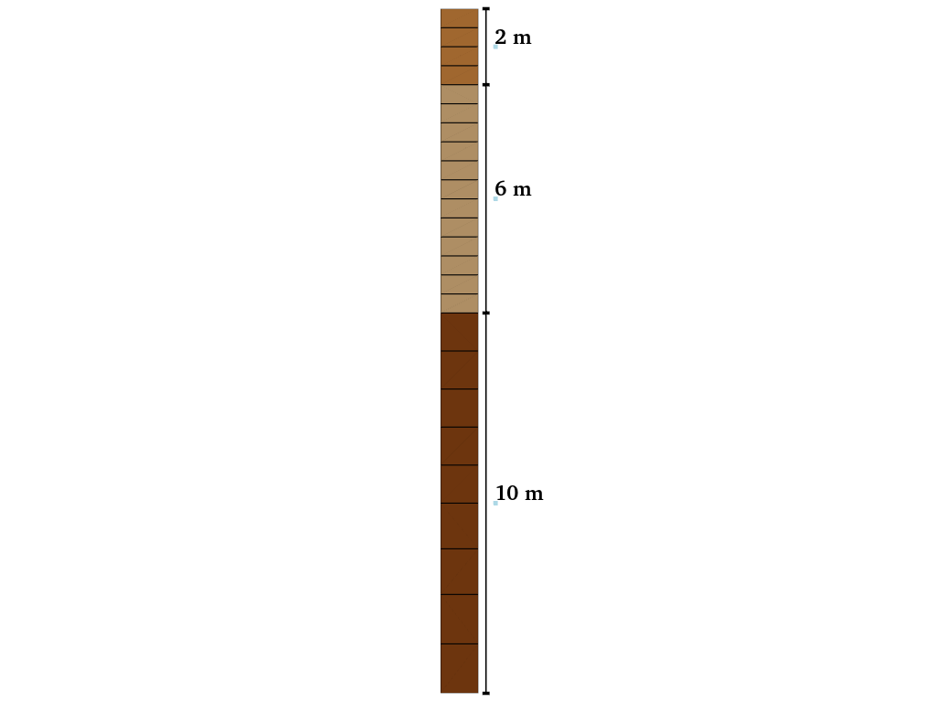
Schematic representation of the multi-layered soil profile used in this example.
Model Description
Soil Column:
Single 1m × 1m soil column in horizontal dimensions
Total depth of 18m
Three distinct soil layers with different material properties:
Layer 1: 10m thick (bottom) - Stiff material
Layer 2: 6m thick (middle) - Medium stiffness material
Layer 3: 2m thick (top) - Soft material
Materials:
Unlike Example 1 which used a single material with uniform properties, this example uses three distinct materials:
Layer 1 (Bottom):
Shear wave velocity (Vs): 262.5 m/s
Unit weight (γ): 19.9 kN/m³
Rayleigh damping: 3% at frequencies 2.76Hz and 13.84Hz
Layer 2 (Middle):
Shear wave velocity (Vs): 196.3 m/s
Unit weight (γ): 19.1 kN/m³
Rayleigh damping: 3% at frequencies 2.76Hz and 13.84Hz
Layer 3 (Top):
Shear wave velocity (Vs): 144.3 m/s
Unit weight (γ): 19.8 kN/m³
Rayleigh damping: 3% at frequencies 2.76Hz and 13.84Hz
Mesh, Loading, and Analysis:
These aspects remain similar to Example 1, with appropriate adjustments for the different layer configuration.
Implementation Details
Let’s focus on the key differences in implementation compared to Example 1:
Material Definition with Multiple Properties
Unlike Example 1 which used identical material properties, this example defines three distinct materials:
# Material properties for three distinct layers
layer1 = {
    "vs": 262.5199305117452,  # Shear wave velocity in m/s
    "rho": 19.9*1000/9.81,    # Density in kg/m³
    "damping": 0.03,          # Damping ratio
}

layer2 = {
    "vs": 196.2675276462639,  # Shear wave velocity in m/s
    "rho": 19.1*1000/9.81,    # Density in kg/m³
    "damping": 0.03,          # Damping ratio
}

layer3 = {
    "vs": 144.2535646321813,  # Shear wave velocity in m/s
    "rho": 19.8*1000/9.81,    # Density in kg/m³
    "damping": 0.03,          # Damping ratio
}
For each layer, the shear modulus is calculated based on the shear wave velocity and density:
# Calculate shear modulus and other derived properties for each layer
for layer in [layer1, layer2, layer3]:
    rho = layer["rho"]
    Vs = layer["vs"]
    G = rho * Vs**2        # Shear modulus in Pa
    nu = 0.3               # Assumed value for Poisson's ratio
    E = 2 * G * (1 + nu)   # Young's modulus in Pa
    layer["E"] = E / 1000. # Convert to kPa
    layer["nu"] = nu
    layer["rho_model"] = rho / 1000. # Convert to t/m³
Layer Definition and Mesh Generation
The soil column is modeled as a stack of three layers with varying properties:
# Create the three material types with different properties
fm.material.create_material(material_category="nDMaterial", material_type="ElasticIsotropic",
                          user_name="Bottom Layer",  E=layer1["E"], nu=layer1["nu"], rho=layer1["rho_model"])

fm.material.create_material(material_category="nDMaterial", material_type="ElasticIsotropic",
                          user_name="Middle Layer",  E=layer2["E"], nu=layer2["nu"], rho=layer2["rho_model"])

fm.material.create_material(material_category="nDMaterial", material_type="ElasticIsotropic",
                          user_name="Top Layer", E=layer3["E"], nu=layer3["nu"], rho=layer3["rho_model"])

# Create elements with different material properties
BottomEle = fm.element.create_element(element_type="stdBrick", ndof=3,
                                    material="Bottom Layer",
                                    b1=0.0, b2=0.0, b3=-9.81 * layer1["rho_model"])

MiddleEle = fm.element.create_element(element_type="stdBrick", ndof=3,
                                    material="Middle Layer",
                                    b1=0.0, b2=0.0, b3=-9.81 * layer2["rho_model"])

TopEle = fm.element.create_element(element_type="stdBrick", ndof=3,
                                  material="Top Layer",
                                  b1=0.0, b2=0.0, b3=-9.81 * layer3["rho_model"])
Using the TransferFunction Class for Analytical Solutions
A key feature of this example is the use of Femora’s built-in TransferFunction class to calculate analytical solutions. This helper class, located in the femora.tools module, provides a convenient way to compute the theoretical transfer function for layered soil profiles.
In Example 1, we manually calculated the analytical transfer function using mathematical formulas. In this example, we leverage the TransferFunction class to handle the complexity of multi-layered calculations:
from femora.tools.transferFunction import TransferFunction

# Define soil profile from top to bottom
soil = [
    {"h": 2,  "vs": 144.2535646321813, "rho": 19.8*1000/9.81, "damping": 0.03,
     "damping_type":"rayleigh", "f1": 2.76, "f2": 13.84},
    {"h": 6,  "vs": 196.2675276462639, "rho": 19.1*1000/9.81, "damping": 0.03,
     "damping_type":"rayleigh", "f1": 2.76, "f2": 13.84},
    {"h": 10, "vs": 262.5199305117452, "rho": 19.9*1000/9.81, "damping": 0.03,
     "damping_type":"rayleigh", "f1": 2.76, "f2": 13.84},
]

# Define rock half-space properties
rock = {"vs": 8000, "rho": 2000.0, "damping": 0.00}

# Create transfer function object and compute
tf = TransferFunction(soil_profile=soil, rock=rock, f_max=22)
f, TF, _ = tf.compute()

# Plot the results
import matplotlib.pyplot as plt
import numpy as np
plt.figure(figsize=(10, 5))
plt.plot(f, np.abs(TF))
plt.xlabel("Frequency (Hz)")
plt.show()
The beauty of this approach is that we can use exactly the same soil properties in both our numerical model and analytical calculation. This ensures an apples-to-apples comparison between the Femora finite element solution and the theoretical transfer function.
The TransferFunction class handles all the complex mathematics of the transfer matrix method, including:
Calculating the complex impedance for each layer
Applying the appropriate damping model (constant or Rayleigh)
Computing wave propagation through multiple interfaces
Accounting for frequency-dependent behavior
This tool makes it easy to verify numerical results against theoretical solutions, which is particularly valuable when developing more complex models.
Results and Analysis
The transfer function comparison for this example demonstrates the accuracy of Femora in modeling wave propagation through multiple soil layers with different properties:
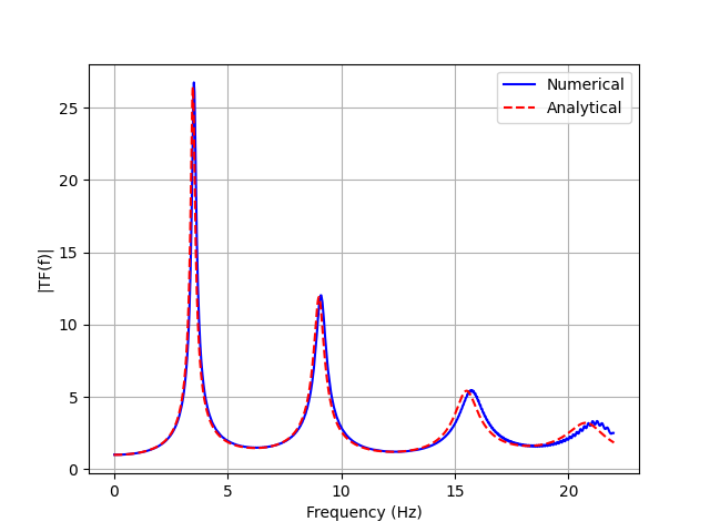
Comparison of numerical (blue) and analytical (red) transfer functions for the three-layer soil profile
The analytical transfer function is calculated using the TransferFunction class from Femora, which implements the solution for one-dimensional wave propagation through multiple elastic layers with frequency-dependent damping.
Effect of Layer Properties on Site Response
The multi-layered soil profile results in greater amplification and shifts in resonance frequencies compared to the uniform soil column in Example 1:
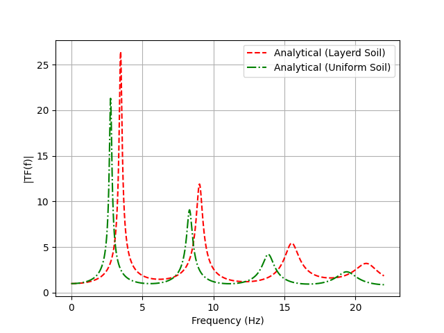
Comparison of transfer functions between uniform soil (Example 1) and multi-layered soil (Example 2)
Simulation Visualization
This animation demonstrates:
The change in wave propagation velocity as waves move through different material layers
The reflection and refraction of waves at layer interfaces
The complex resonance patterns resulting from the impedance contrasts between layers
Conclusion
This example demonstrates:
How to model a multi-layered soil profile with varying material properties in Femora
How to use the
TransferFunctionclass to calculate analytical solutions for complex soil profilesThe importance of accurately modeling layer properties for site response analysis
The validation of numerical results against analytical solutions for multi-layered soil
The combination of numerical simulation with analytical verification provides confidence in Femora’s ability to accurately model site response for complex soil conditions.
Code Access
The full source code for this example is available in the Femora repository:
Example directory:
examples/SiteResponse/Example2/Python script:
examples/SiteResponse/Example2/femoramodel.pyTransfer function script:
examples/SiteResponse/Example2/TransferFunction.pyPost-processing script:
examples/SiteResponse/Example2/plot.py
Below is the complete code for this example:
import os
import femora as fm
os.chdir(os.path.dirname(__file__))


# create one damping for all the meshParts
uniformDamp = fm.damping.frequencyRayleigh(f1 = 2.76, f2 = 13.84, dampingFactor=0.03)
region = fm.region.elementRegion(damping=uniformDamp)

# defining the mesh parts
Xmin = 0.0 ;Xmax = 1.0
Ymin = 0.0 ;Ymax = 1.0
Zmin = -18.;Zmax = 0.0
dx   = 1.0; dy   = 1.0
Nx = int((Xmax - Xmin)/dx)
Ny = int((Ymax - Ymin)/dy)


layers_properties = [
    {"user_name": "Dense Ottawa1",  "G": 145.0e6, "gamma": 19.9,  "nu": 0.3, "thickness": 2.6, "dz": 1.3},
    {"user_name": "Dense Ottawa2",  "G": 145.0e6, "gamma": 19.9,  "nu": 0.3, "thickness": 2.4, "dz": 1.2},
    {"user_name": "Dense Ottawa3",  "G": 145.0e6, "gamma": 19.9,  "nu": 0.3, "thickness": 5.0, "dz": 1.0},
    {"user_name": "Loose Ottawa",   "G": 75.0e6,  "gamma": 19.1,  "nu": 0.3, "thickness": 6.0, "dz": 0.5},
    {"user_name": "Dense Montrey",  "G": 42.0e6,  "gamma": 19.8,  "nu": 0.3, "thickness": 2.0, "dz": 0.5}
]


for layer in layers_properties:
    name = layer["user_name"]
    nu   = layer["nu"]
    rho  = layer["gamma"] * 1000 / 9.81        # Density in kg/m^3
    Vs   = (layer["G"] / rho) ** 0.5           # Shear wave velocity in m/s
    E    = 2 * layer["G"] * (1 + layer["nu"])  # Young's modulus in Pa
    E    = E / 1000.                           # Convert to kPa
    rho  = rho / 1000.                         # Convert to kg/m^3

    print(f"Layer: {name}, Vs: {Vs}")


    # Define the material
    fm.material.create_material(material_category="nDMaterial", material_type="ElasticIsotropic", user_name=name, E=E, nu=nu, rho=rho)

    # Define the element
    ele = fm.element.create_element(element_type="stdBrick", ndof=3, material=name, b1=0.0, b2=0.0, b3=-9.81 * rho)

    fm.meshPart.create_mesh_part(category="Volume mesh", mesh_part_type="Uniform Rectangular Grid",
                                 user_name=name, element=ele, region=region,
                                **{
                                    'X Min': Xmin, 'X Max': Xmax,
                                    'Y Min': Ymin, 'Y Max': Ymax,
                                    'Z Min': Zmin, 'Z Max': Zmin + layer["thickness"],
                                    'Nx Cells': Nx, 'Ny Cells': Ny, 'Nz Cells': int(layer["thickness"] / layer["dz"])
                                })
    Zmin += layer["thickness"]


# #  Create assembly Sections
fm.assembler.create_section(meshparts=[layer["user_name"] for layer in layers_properties], num_partitions=0)


# Assemble the mesh parts
fm.assembler.Assemble()

# Create a TimeSeries for the uniform excitation
timeseries = fm.timeSeries.create_time_series(series_type="path",
                                              filePath="FrequencySweep.acc",
                                              fileTime="FrequencySweep.time",
                                              factor= 9.81)

# Create a pattern for the uniform excitation
kobe = fm.pattern.create_pattern(pattern_type="uniformexcitation",dof=1, time_series=timeseries)


# boundary conditions
fm.constraint.mp.create_laminar_boundary(bounds=(-17.9,0),dofs=[1,2,3], direction=3)
fm.constraint.sp.fixMacroZmin(dofs=[1,1,1],tol=1e-3)


# Create a recorder for the whole model
mkdir = fm.actions.tcl("file mkdir Results")
recorder = fm.recorder.create_recorder("vtkhdf", file_base_name="Results/result.vtkhdf",resp_types=["accel", "disp"], delta_t=0.001)

# gravity analysis
newmark_gamma = 0.6
newnark_beta = (newmark_gamma + 0.5)**2 / 4
system = fm.analysis.system.bandGeneral()
numberer = fm.analysis.numberer.rcm()
dampNewmark = fm.analysis.integrator.newmark(gamma=newmark_gamma, beta=newnark_beta)
gravity = fm.analysis.create_default_transient_analysis(username="gravity",
                                                        dt=1.0, num_steps=30,
                                                        options={"system": system,
                                                                 "numberer": numberer,
                                                                 "integrator": dampNewmark})

# dynamic analysis
dynamic = fm.analysis.create_default_transient_analysis(username="dynamic",
                                                        final_time=50.0, dt=0.001,
                                                        options={"system": system,
                                                                 "numberer": numberer})


reset = fm.actions.seTime(pseudo_time=0.0)

# Add the recorder and gravity analysis step to the process
fm.process.add_step(gravity,  description="Gravity Analysis Step")
fm.process.add_step(kobe,     description="Uniform Excitation (Kobe record)")
fm.process.add_step(mkdir,    description="Create Results Directory")
fm.process.add_step(recorder, description="Recorder of the whole model")
fm.process.add_step(reset,    description="Reset pseudo time")
fm.process.add_step(dynamic,  description="Dynamic Analysis Step")
fm.export_to_tcl("mesh.tcl")


# fm.gui()