Example 1: Domain Reduction Method (DRM) Site Response Analysis
Overview
This example demonstrates the Domain Reduction Method (DRM) implementation in Femora for site response analysis. Building upon the foundation established in Site Response Examples 3 and 4, this example shows how to:
Use the deconvolved bedrock motion from Site Response Example 4 as DRM input
Apply the 3D mesh configuration from Site Response Example 3 for DRM analysis
Create and apply DRM load patterns using the
TransferFunctiontoolConfigure absorbing boundary layers for realistic wave absorption
Compare DRM results with analytical solutions and previous site response analyses
The DRM approach provides a more realistic representation of seismic wave propagation by applying motion at interior boundaries rather than uniform base excitation, making it particularly valuable for complex site response and soil-structure interaction problems.
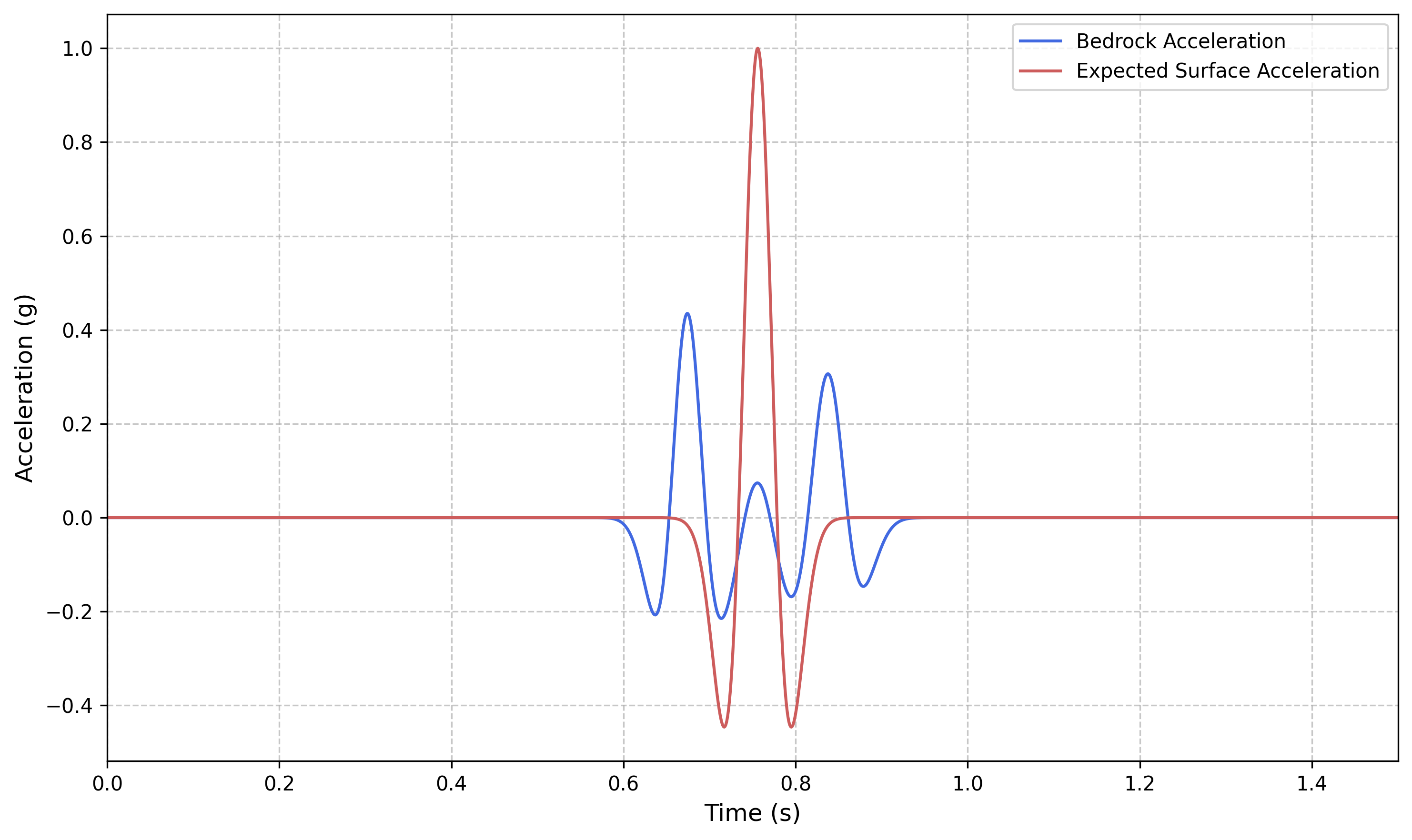
Bedrock acceleration input (computed via deconvolution in Site Response Example 4) and expected surface response
Model Description
Relationship to Previous Examples:
This example combines key elements from two previous site response examples:
From Site Response Example 3: The 3D mesh configuration (10m × 10m × 18m domain) with multi-layer soil profile
From Site Response Example 4: The deconvolved bedrock motion (Ricker wavelet) obtained through transfer function analysis
Soil Profile:
The model uses the same three-layer soil profile as Examples 2-4:
Layer 1 (Top): 2.6m thick - Dense Ottawa sand (Vs = 262.5 m/s)
Layer 2 (Middle): 8.0m thick - Medium density material (Vs = 196.3 m/s)
Layer 3 (Bottom): 7.4m thick - Loose Ottawa sand (Vs = 144.3 m/s)
All layers include frequency-dependent Rayleigh damping with the same parameters as previous examples (f1 = 2.76 Hz, f2 = 13.84 Hz, ζ = 3%).
Domain Configuration:
Horizontal dimensions: 10m × 10m (identical to Site Response Example 3)
Vertical extent: 18m depth (same as all site response examples)
Mesh discretization: 1m × 1m horizontal elements with variable vertical spacing
Parallel processing: 4 partitions for distributed computation
Domain Reduction Method Implementation
The DRM implementation in this example introduces several new concepts not covered in the site response examples:
Creating the DRM Load Pattern
The key innovation in this example is the creation of DRM load patterns using the TransferFunction class. This process involves several steps that are unique to DRM analysis:
from femora.tools.transferFunction import TransferFunction, TimeHistory

# Load the deconvolved bedrock motion from Site Response Example 4
record = TimeHistory.load(acc_file="ricker_base.acc",
                          time_file="ricker_base.time",
                          unit_in_g=True,
                          gravity=9.81)

# Create transfer function instance with soil profile
tf = TransferFunction(soil, rock, f_max=50.0)

# Extract the assembled mesh for DRM pattern creation
mesh = fm.assembler.get_mesh()

# Create DRM pattern - this is the key new functionality
tf.createDRM(mesh, props={"shape":"box"},
             time_history=record, filename="drmload.h5drm")
The createDRM method performs several critical operations:
Mesh Analysis: Identifies boundary nodes that will receive DRM forces
Wave Field Computation: Calculates the theoretical wave field throughout the domain
Force Calculation: Computes equivalent nodal forces for DRM implementation
HDF5 Output: Writes the DRM load pattern to an HDF5 file for efficient loading
Applying the DRM Pattern
Once the DRM load pattern is created, it’s applied to the model using Femora’s pattern system:
# Create H5DRM pattern object
h5pattern = fm.pattern.create_pattern('h5drm',
                                     filepath='drmload.h5drm',
                                     factor=1.0,
                                     crd_scale=1.0,
                                     distance_tolerance=0.01,
                                     do_coordinate_transformation=1,
                                     transform_matrix=[1.0, 0.0, 0.0, 0.0, 1.0, 0.0, 0.0, 0.0, 1.0],
                                     origin=[0.0, 0.0, 0.0])
This creates a specialized pattern that can read and apply the HDF5-based DRM loads throughout the analysis.
Absorbing Boundary Configuration
A critical component of DRM analysis is the proper configuration of absorbing boundaries to prevent artificial wave reflections:
# Add absorbing layers around the domain
fm.drm.addAbsorbingLayer(numLayers=2,
                        numPartitions=1,
                        partitionAlgo="kd-tree",
                        geometry="Rectangular",
                        rayleighDamping=0.95,
                        matchDamping=False,
                        type="Rayleigh")
This configuration:
numLayers=2: Creates a two-layer absorbing boundary
rayleighDamping=0.95: Applies high damping (95%) in the absorbing region
geometry=”Rectangular”: Configures absorbing boundaries for box-shaped domains
partitionAlgo=”kd-tree”: Uses k-d tree algorithm for efficient boundary identification
DRM Process Configuration
The DRM analysis requires specific process configuration that differs from standard site response analysis:
# Set the DRM pattern
fm.drm.set_pattern(h5pattern)

# Create DRM-specific analysis process
fm.drm.createDefaultProcess(finalTime=2.0, dT=0.005,
                           vtkhdfrecorder_delta_t=0.005,
                           vtkhdfrecorder_file=f"{resultdirectoryname}/result")
This creates a complete analysis process specifically configured for DRM analysis, including:
Time integration parameters optimized for DRM
Output recorders configured for DRM visualization
Proper sequencing of DRM load application
Results and Analysis
Transfer Function Validation
The transfer function comparison demonstrates that the DRM method accurately reproduces the expected site response:
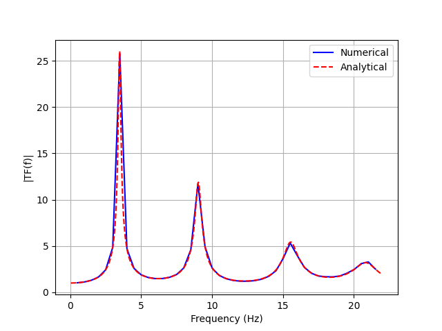
Comparison of analytical transfer function with DRM numerical results
The excellent agreement between the analytical and DRM numerical results validates:
The accuracy of the DRM load pattern generation
The proper implementation of absorbing boundaries
The consistency with previous site response analyses
Time History Comparison
The most comprehensive validation comes from comparing time histories of acceleration, velocity, and displacement:
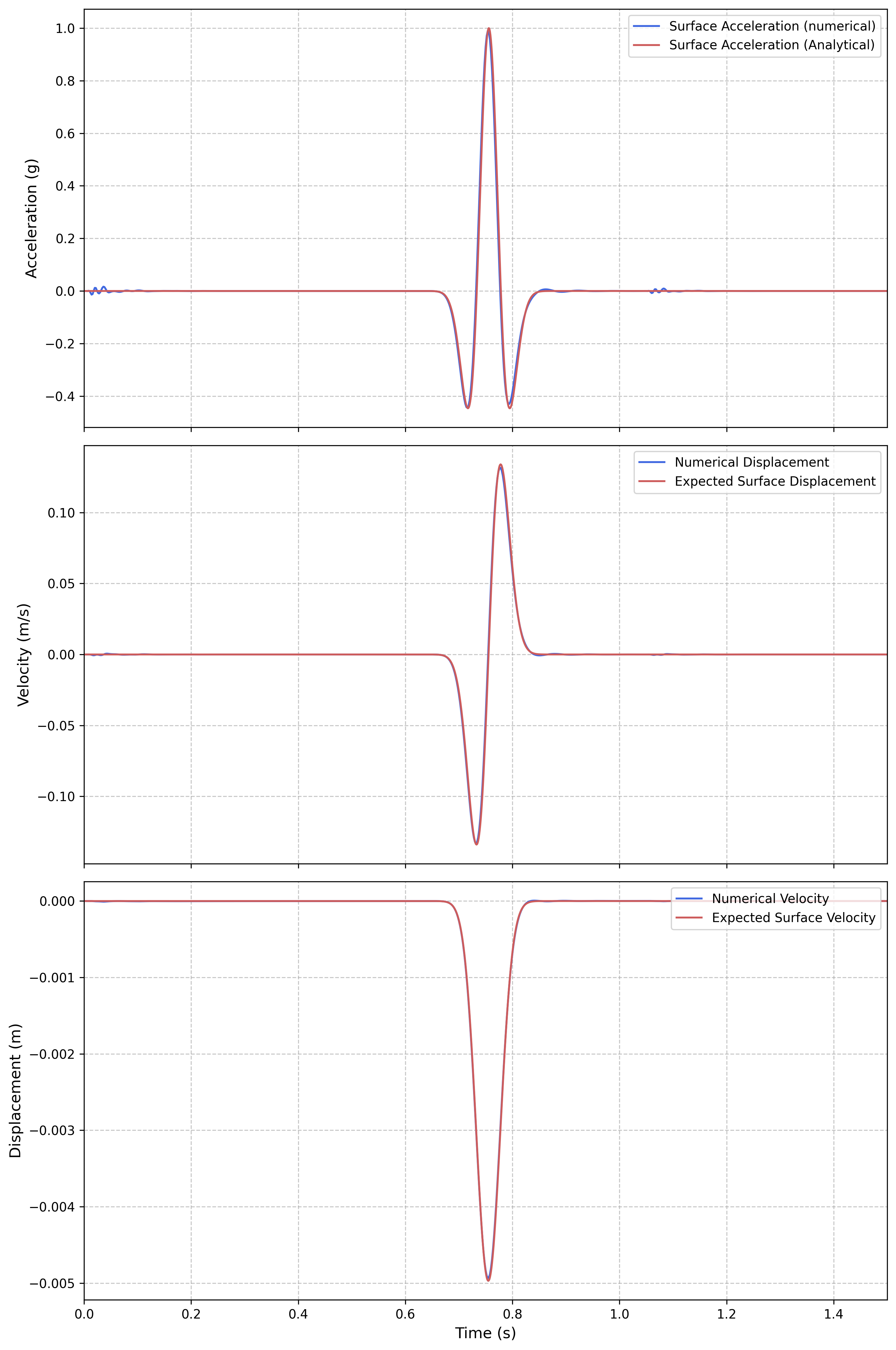
Comparison of numerical DRM results with analytical solutions for acceleration, velocity, and displacement
This comparison shows:
Acceleration: Excellent agreement in both amplitude and phase
Velocity: Consistent integration from acceleration with proper baseline correction
Displacement: Accurate representation of permanent deformation patterns
The close agreement across all response quantities demonstrates the robustness of the DRM implementation.
3D Wave Propagation Visualization
The DRM method provides detailed insight into wave propagation through the 3D domain:
This animation shows:
Shear Stress Contours: Distribution of shear stress throughout the deformed domain
Wave Propagation: Realistic wave fronts propagating from the DRM boundary
Layer Effects: Amplification and attenuation effects at layer interfaces
Absorbing Boundaries: Effective wave absorption at domain boundaries
Advantages of DRM Over Uniform Excitation
This example demonstrates several key advantages of the DRM approach compared to the uniform base excitation used in Site Response Examples 1-3:
Physical Realism:
DRM applies motion at interior boundaries, mimicking actual wave propagation
Allows for more complex wave fields including oblique incidence
Enables modeling of finite fault sources and complex source mechanisms
Computational Efficiency:
Smaller computational domains due to effective absorbing boundaries
Reduced artificial reflections from domain boundaries
Better representation of far-field conditions
Flexibility:
Can accommodate complex geometries and topography
Suitable for soil-structure interaction problems
Enables coupling with regional wave propagation models
Relationship to Site Response Examples
This DRM example builds directly on the foundation established in the site response series:
From Site Response Example 3: * 3D mesh configuration and parallel processing setup * Multi-layer soil profile definition and material properties * Visualization and post-processing techniques
From Site Response Example 4:
* Deconvolution methodology using the TransferFunction class
* Bedrock motion calculation from surface recordings
* Time history validation approaches
New Concepts Introduced: * DRM load pattern generation and application * Absorbing boundary layer configuration * HDF5-based load pattern management * DRM-specific analysis process setup
The seamless integration of these concepts demonstrates the modular design of Femora and the consistency of the analysis framework across different seismic analysis methods.
Practical Applications
The DRM methodology demonstrated in this example is particularly valuable for:
Regional Seismic Analysis: * Coupling site-specific models with regional wave propagation simulations * Modeling earthquake scenarios with realistic source mechanisms * Analyzing basin effects and complex 3D wave propagation
Soil-Structure Interaction: * More realistic representation of free-field motion around structures * Reduced computational domain size for large structural systems * Better modeling of structure-induced wave scattering
Advanced Site Response: * Incorporation of topographic effects on site amplification * Modeling of complex layering and lateral variations * Analysis of slope stability under seismic loading
Conclusion
This example demonstrates:
The successful implementation of the Domain Reduction Method in Femora
Integration of deconvolution tools with DRM load pattern generation
Effective use of absorbing boundaries for realistic wave propagation modeling
Validation of DRM results against analytical solutions and previous examples
The DRM approach provides a powerful extension to the site response analysis capabilities demonstrated in the previous examples, offering greater physical realism and computational flexibility for complex seismic analysis problems.
Code Access
The full source code for this example is available in the Femora repository:
Example directory:
examples/DRM/Example1/DRM model script:
examples/DRM/Example1/femoramodel.pyPost-processing script:
examples/DRM/Example1/plot.pyAnimation script:
examples/DRM/Example1/movie.py
The complete model setup code is shown below:
import os
import femora as fm
os.chdir(os.path.dirname(__file__))


# create one damping for all the meshParts
uniformDamp = fm.damping.frequencyRayleigh(f1 = 2.76, f2 = 13.84, dampingFactor=0.03)
region = fm.region.elementRegion(damping=uniformDamp)

# defining the mesh parts
Xmin = -5.0 ;Xmax = 5.0
Ymin = -5.0 ;Ymax = 5.0
Zmin = -18.;Zmax = 0.0
dx   = 1.0; dy   = 1.0
Nx = int((Xmax - Xmin)/dx)
Ny = int((Ymax - Ymin)/dy)


layers_properties = [
    {"user_name": "Dense Ottawa1",  "G": 145.0e6, "gamma": 19.9,  "nu": 0.3, "thickness": 2.6, "dz": 1.3},
    {"user_name": "Dense Ottawa2",  "G": 145.0e6, "gamma": 19.9,  "nu": 0.3, "thickness": 2.4, "dz": 1.2},
    {"user_name": "Dense Ottawa3",  "G": 145.0e6, "gamma": 19.9,  "nu": 0.3, "thickness": 5.0, "dz": 1.0},
    {"user_name": "Loose Ottawa",   "G": 75.0e6,  "gamma": 19.1,  "nu": 0.3, "thickness": 6.0, "dz": 0.5},
    {"user_name": "Dense Montrey",  "G": 42.0e6,  "gamma": 19.8,  "nu": 0.3, "thickness": 2.0, "dz": 0.5}
]


for layer in layers_properties:
    name = layer["user_name"]
    nu   = layer["nu"]
    rho  = layer["gamma"] * 1000 / 9.81        # Density in kg/m^3
    Vs   = (layer["G"] / rho) ** 0.5           # Shear wave velocity in m/s
    E    = 2 * layer["G"] * (1 + layer["nu"])  # Young's modulus in Pa
    E    = E / 1000.                           # Convert to kPa
    rho  = rho / 1000.                         # Convert to kg/m^3

    print(f"Layer: {name}, Vs: {Vs}")


    # Define the material
    fm.material.create_material(material_category="nDMaterial", material_type="ElasticIsotropic", user_name=name, E=E, nu=nu, rho=rho)

    # Define the element
    ele = fm.element.create_element(element_type="stdBrick", ndof=3, material=name, b1=0.0, b2=0.0, b3=0.0)

    fm.meshPart.create_mesh_part(category="Volume mesh", mesh_part_type="Uniform Rectangular Grid",
                                 user_name=name, element=ele, region=region,
                                **{
                                    'X Min': Xmin, 'X Max': Xmax,
                                    'Y Min': Ymin, 'Y Max': Ymax,
                                    'Z Min': Zmin, 'Z Max': Zmin + layer["thickness"],
                                    'Nx Cells': Nx, 'Ny Cells': Ny, 'Nz Cells': int(layer["thickness"] / layer["dz"])
                                })
    Zmin += layer["thickness"]


#  Create assembly Sections
fm.assembler.create_section(meshparts=[layer["user_name"] for layer in layers_properties], num_partitions=4)


# Assemble the mesh parts
fm.assembler.Assemble()

# ===================================================================
# creating the DRM pattern
# ===================================================================

# the soil layers is equivalent to the mesh parts defined above
# this is baisc format that the transfer function will use
soil = [
    {"h": 2,  "vs": 144.2535646321813, "rho": 19.8*1000/9.81, "damping": 0.03, "damping_type":"rayleigh", "f1": 2.76, "f2": 13.84},
    {"h": 6,  "vs": 196.2675276462639, "rho": 19.1*1000/9.81, "damping": 0.03, "damping_type":"rayleigh", "f1": 2.76, "f2": 13.84},
    {"h": 10, "vs": 262.5199305117452, "rho": 19.9*1000/9.81, "damping": 0.03, "damping_type":"rayleigh", "f1": 2.76, "f2": 13.84},
]

# the rock layer is defined as a single layer with the properties below
# we just assume a hard rock layer with high shear wave velocity and density
# to represent the rigid base condition to create a high impedance contrast
rock = {"vs": 8000, "rho": 2000.0, "damping": 0.00}

from femora.tools.transferFunction import TransferFunction, TimeHistory


# Create TimeHistory instance
# for the DRM pattern we need to provide a time history of the ground motion
# in this case we use a Ricker wavelet based ground motion that we calculate using deconvolution of ricker wavelet
# at the surface of the soil layers to compute the time history of the base motion
record = TimeHistory.load(acc_file="ricker_base.acc",
                            time_file="ricker_base.time",
                            unit_in_g=True,
                            gravity=9.81)


# Create transfer function instance
# initialize the transfer function with the soil layers and rock properties
# the f_max is the maximum frequency of the transfer function
tf = TransferFunction(soil, rock, f_max=50.0)


# Create DRM pattern
# for creating the DRM pattern we need to provide the mesh (pyvista mesh),
# the properties of the DRM pattern (shape, time history, filename)
# the mesh is the final that we assembled above lest extraxted mesh from the assembled model
mesh = fm.assembler.get_mesh()

# now we can create the DRM pattern using the transfer function and the mesh
# since we our mesh is box shaped we can use the box shape for the DRM pattern
# to the date of this writing the DRM pattern is only supported for box shaped meshes
# the box shape mesh should be representation of the soil box should start at z=0 and extend to the depth  with negative z values
tf.createDRM(mesh, props={"shape":"box"}, time_history=record, filename="drmload.h5drm")

h5pattern = fm.pattern.create_pattern( 'h5drm',
                                        filepath='drmload.h5drm',
                                        factor=1.0,
                                        crd_scale=1.0,
                                        distance_tolerance=0.01,
                                        do_coordinate_transformation=1,
                                        transform_matrix=[1.0, 0.0, 0.0, 0.0, 1.0, 0.0, 0.0, 0.0, 1.0],
                                        origin=[0.0, 0.0, 0.0])
# ===================================================================
# ===================================================================
fm.drm.addAbsorbingLayer(numLayers=2,
                        numPartitions=1,
                        partitionAlgo="kd-tree",
                        geometry="Rectangular",
                        rayleighDamping=0.95,
                        matchDamping=False,
                        type="Rayleigh",
                        )
fm.drm.set_pattern(h5pattern)
fm.drm.createDefaultProcess(finalTime=30, dT=0.01)

resultdirectoryname = "Results"
fm.process.insert_step(index=0, component=fm.actions.tcl(f"file mkdir {resultdirectoryname}"), description="making result directory")

fm.export_to_tcl(filename="model.tcl")